Protostar synthetic spectrum
In this section, we introduce the protostar synthetic spectrum calculator. This tool aims to support the interpretation of JWST observations. The steps through the construction of the synthetic spectrum are described below as well as the link with JWST/ETC calculator.
Setting up the interpolation range
This online tool uses data of several ice spectra as well as of spectral energy distribution (SED) of protostars. These data often have different resolution, and therefore, they need to be interpolated to be treated consistently through out mathematical operations.
When the range provided to the tool is out of the boundaries of the data hosted in the database, the user is notified and instructed to add different ranges, as shown in Figure 1.

Figure 1: Boundary error notification.
Selecting the ice spectra
All absorbance spectra hosted in the Leiden Ice Database can be accessed via this online tool. By clicking on the Analogue field, the user will see a dropdown with the ice analogues available, as shown in Figure 2:
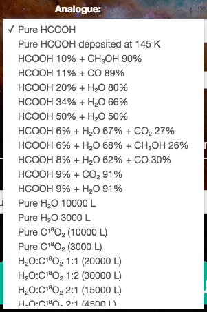
Figure 2: Dropdown menu for selection of ice analogues.
When the ice analogue is selected, the temperature options are automatically load in the field Temperature, as show in Figure 3.
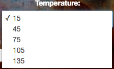
Figure 3: Dropdown menu for selection of the spectrum temperature.
Defining ice column density
After selecting the ice analogue and temperature, the user must provide the ice column density. The input provided in the field Column density (\(N_{ice}^{input}\)) is used to create a scale factor, defined as:
where \(N_{ice}^{lab}\) is the ice column density of the experimental data. The scaling factor \(w\) is a factor to increase or decrease the ice column density of the selected analogue.
Optical depth spectrum
The IR absorbance spectra of ices are converted to an optical depth scale after the column density is provided. The reason for this conversion is that astronomical spectra toward protostars are often converted to optical depth scale for comparison with experimental data. The conversion from absorbance (\(Abs\)) to optical depth is performed by:
When more than one ice analogue is selected, the total spectrum in optical depth scale is obtained with a linear combination of all components. Figure 4 shows an optical depth synthetic spectrum after the combination of three ice analogues and the silicate from the astronomical source GCS3.

Figure 4: Synthetic spectrum in optical depth scale.
Selecting the SED continuum
Now that the optical depth synthetic spectrum has been created, the user can go one step forward and simulate the spectrum of a protostar in flux scale, i.e., in Jy units (\(F_{\lambda}^{synth}\)). To do this step, SPECFY uses the following equation:
where \(F_{\lambda}^{cont}\) is the continuum SED toward the protostar and \(\tau_{\lambda}\) is the synthetic optical depth spectrum created before. To make this step simple, a few continuum SED were compiled from Boogert et al. (2008). For more details about the methodology used, please, check out the paper and Rocha et al. (in prep.).
As an example, the optical depth spectrum in Figure 4 is converted to Flux scale by using the continuum SED of the protostar Elias 29. The result is shown in Figure 5.

Figure 5: Synthetic spectrum with ice absorption bands. Continuum SED from Elias 29 protostar.
Downloading the results
The plots can be downloaded by using the save tool in the Bokeh toolbar. To download the files with the data, please use the green button labeled Download the synthetic spectrum.
Synergy: connecting SPECFY with the JWST/Exposure Time Calculator
Under construction…